Level 03: Deep Revolution

The Promise of Deep Networks

In Level 2, you learned about neural networks. But here's the exciting part: the more layers you add, the more powerful the network becomes! At least, that's what everyone thought...

            The Intuition: Early layers learn simple features (edges, colors). 
            Middle layers combine them (shapes, textures). Deep layers combine those (objects, faces). 
            More layers = more complex understanding!
          

Imagine trying to recognize a cat:

Input: Raw Pixels 1920×1080×3 numbers

↓

Output: "It's a cat!" 99.7% confident

This hierarchical learning seems perfect. So researchers kept adding layers: 10, 20, 50, 100... But something went terribly wrong.

Hierarchical Feature Learning

Deep neural networks exhibit a remarkable property: hierarchical feature extraction. Lower layers learn low-level features, while deeper layers compose these into higher-level abstractions.

Feature Hierarchy in Vision

Layers 1-2: Edge detectors (Gabor-like filters)
Layers 3-4: Texture detectors, simple patterns
Layers 5-6: Object parts (eyes, wheels, corners)
Layers 7+: Complete objects, semantic concepts

This compositional structure suggests that deeper networks—with more layers—should achieve better performance by learning increasingly abstract representations.

The Depth Hypothesis

Prior to 2015, the prevailing wisdom was: deeper is better. Theoretically, a deep network can represent any function a shallow network can, with exponentially fewer parameters (Eldan & Shamir, 2016).

However, practical training of deep networks encountered a fundamental obstacle.

The Problem: Vanishing Gradients

Remember backpropagation from Level 2? Gradients flow backward through the network, telling each layer how to adjust its weights. But in deep networks, something terrible happens:

            The Vanishing Gradient Problem: In deep networks, gradients become 
            extremely small by the time they reach early layers. Those layers barely learn at all!
          

Why does this happen? It comes down to the chain rule. Remember, we multiply gradients together as we go backward through the network. When you multiply many small numbers together, they get really small:

📉 Gradient Flow in a Deep Network

Watch how gradients shrink as we go backward through layers:

Output

1.0

Layer 10

0.8

Layer 20

0.02

Layer 30

0.0001

Layer 50

~0

Result: Early layers learn almost nothing. The network effectively becomes shallow, wasting all those extra layers!

Gradient Vanishing in Deep Networks

The vanishing gradient problem arises from the nature of backpropagation in deep architectures. Recall that gradients are computed via the chain rule:

∂L/∂W⁽ˡ⁾ = ∂L/∂a⁽ᴸ⁾ × ∂a⁽ᴸ⁾/∂z⁽ᴸ⁾ × ∂z⁽ᴸ⁾/∂a⁽ᴸ⁻¹⁾ × ... × ∂a⁽ˡ⁺¹⁾/∂z⁽ˡ⁺¹⁾ × ∂z⁽ˡ⁺¹⁾/∂W⁽ˡ⁾

For a network with L layers, the gradient involves multiplying L Jacobian matrices together. With sigmoid or tanh activations (whose derivatives are ≤ 0.25), repeated multiplication causes exponential decay:

If |∂a/∂z| < 1 for all layers, then gradient magnitude ≈ (0.25)^L

Mathematical Analysis

For a layer with sigmoid activation:

Maximum derivative: σ'(0) = 0.25
At saturation: σ'(±∞) → 0
After n layers: gradient < (0.25)^n

With 20 layers, maximum gradient magnitude: (0.25)^20 ≈ 9×10^(-13)—essentially zero for practical purposes.

Consequences

Early layers receive negligible gradient signals
Network fails to learn hierarchical features
Deeper networks perform worse than shallow ones
Training stalls or becomes unstable

The Deep Learning Crisis of 2015

By 2015, researchers were hitting a wall. They tried everything:

✅ Better initialization schemes
✅ Batch normalization (helped!)
✅ Different activation functions (ReLU helped!)
✅ Better optimizers (Adam helped!)
❌ But deep networks still couldn't train reliably beyond ~20 layers

            The Paradox: Shallow networks (10-20 layers) worked fine. 
            Very deep networks (50+ layers) should work better in theory, but they actually performed 
            worse in practice—not just failing to improve, but getting worse!
          

It seemed like deep learning had hit a fundamental limit. Until Microsoft Research published a paper that changed everything...

The Degradation Problem

He et al. (2015) identified that the issue wasn't just vanishing gradients—there was a more fundamental problem they called the degradation problem:

"With the network depth increasing, accuracy gets saturated (which might be unsurprising) and then degrades rapidly. Unexpectedly, such degradation is not caused by overfitting, and adding more layers to a suitably deep model leads to higher training error."

This was shocking because:

The deeper model had more parameters (higher capacity)
The deeper model could simulate the shallow one (by learning identity mappings)
Yet the deeper model performed worse on training data

The problem wasn't model capacity—it was the optimization difficulty of learning the target function.

The ResNet Revolution

Figure 1 from the Paper: Residual Connection

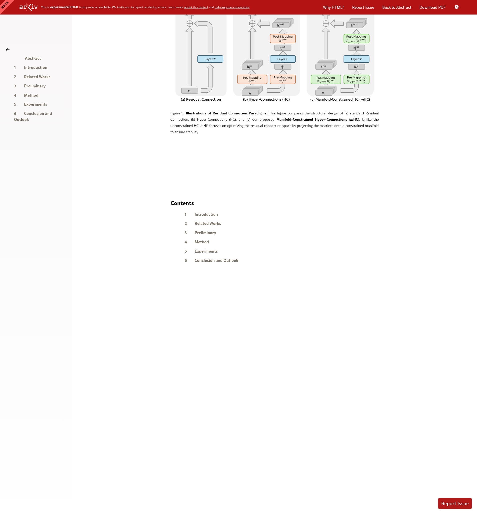
Compare: (a) Standard connection, (b) Hyper-Connections, (c) mHC (from the mHC paper)

The breakthrough idea was shockingly simple: skip connections.

🔄 How Residual Connections Work

Input x

→

Layers
Learn F(x)

+

Skip x

=

Output
F(x) + x

              The Magic Formula: Instead of learning H(x) directly, 
              the network learns F(x) = H(x) - x, and outputs F(x) + x.
              
              This means the network only needs to learn the difference from the input, 
              not the full transformation!

Why This Fixes Everything

With skip connections, gradients can flow directly through the network:

Identity shortcut: Even if all weights are zero, the network passes information through unchanged: output = 0 + x = x
Gradient highway: Gradients can skip layers entirely, preventing vanishing
Easier learning: Network only needs to learn "what's different," not everything

The result? Researchers could now train networks with 152, 1000, even 10,000 layers!

Residual Learning Framework

ResNet reframes the learning objective. Instead of learning a desired mapping H(x), residual blocks learn:

F(x) = H(x) − x

The output becomes:

y = F(x, {Wᵢ}) + x

Mathematical Advantages

Identity by default: If F(x) = 0, then y = x. Networks can easily represent identity mappings.
Gradient preservation: The gradient flows through both paths:
∂y/∂x = ∂F/∂x + 1
Even if ∂F/∂x → 0, ∂y/∂x ≈ 1, preventing vanishing gradients.
Ensemble behavior: ResNets implicitly ensemble many shallow paths (Veit et al., 2016).

Impact

ResNet won the ImageNet 2015 competition with 152 layers—8× deeper than previous winners. More importantly, it enabled the modern era of deep learning, with models now routinely having hundreds or thousands of layers.

What You Learned

            🎓 Key Takeaways
            Deep networks should be better but weren't due to vanishing gradients
Vanishing gradients: Gradients shrink to near-zero in early layers
ResNet solution: Skip connections preserve gradient flow
Identity mapping: Output = F(x) + x, learning only the difference
Result: Networks with 100+ layers became trainable!

          

But here's the thing: ResNet was just the beginning. Researchers kept pushing, trying even more complex connection patterns. Which brings us to the next challenge...

            Summary: From Shallow to Deep
            Hierarchical learning: Deep layers should capture abstract features
Vanishing gradients: Chain rule causes exponential gradient decay
Degradation problem: Deep networks perform worse, not due to overfitting
Residual connections: y = F(x) + x enables identity mappings
Gradient flow: Skip connections provide gradient highways

          

Next: We explore extensions to residual connections—Hyper-Connections—and the challenges they introduce, leading to the mHC solution.